Variational autoencoders
Variational autoencoders
Definition
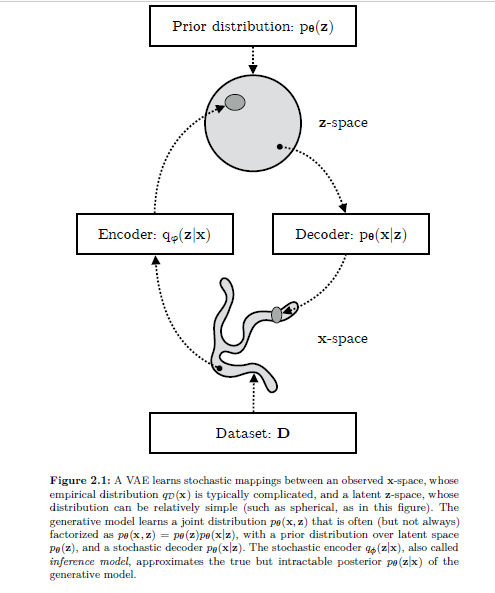
For variational auto-encoders, instead of a deterministic mapping to the latent representation, we model a probability distribution of the latent variable. See figure below from Kingma and Welling 2019
ELBO
We wish to maximise the marginal likelihood of x given by the model. However, this is intractable (as requires integration over the latent variables). Instead we maximise the evidence lower bound, which can be derived by:
\[\begin{aligned} \log p_{\theta}(\mathrm{x})=& \mathbb{E_{q_{\phi}(\mathbf{z} \mid \mathbf{x})}}\left[\log p_{\theta}(\mathrm{x})\right] \\ =& \mathbb{E_{q_{\phi}(\mathbf{z} \mid \mathbf{x})}}\left[\log \left[\frac{p_{\theta}(\mathbf{x}, \mathbf{z})}{p_{\theta}(\mathbf{z} \mid \mathbf{x})}\right]\right] \\ =& \mathbb{E_{q_{\phi}(\mathbf{z} \mid \mathbf{x})}}\left[\log \left[\frac{p_{\theta}(\mathbf{x}, \mathbf{z})}{q_{\phi}(\mathbf{z} \mid \mathbf{x})} \frac{q_{\phi}(\mathbf{z} \mid \mathbf{x})}{p_{\theta}(\mathbf{z} \mid \mathbf{x})}\right]\right] \\ =& \underbrace{\mathbb{E_{q_{\phi}(\mathbf{z} \mid \mathbf{x})}}\left[\log \left[\frac{p_{\theta}(\mathbf{x}, \mathbf{z})}{q_{\phi}(\mathbf{z} \mid \mathbf{x})}\right]\right]}_{=\mathcal{L}_{\theta, \phi}(\mathbf{x}) = (\mathrm{ELBO})}+\underbrace{\mathbb{E_{q_{\phi}(\mathbf{z} \mid \mathbf{x})}}\left[\log \left[\frac{q_{\phi}(\mathbf{z} \mid \mathbf{x})}{p_{\theta}(\mathbf{z} \mid \mathbf{x})}\right]\right]}_{=D_{K L}\left(q_{\phi}(\mathbf{z} \mid \mathbf{x})|| p_{\boldsymbol{\theta}}(\mathbf{z} \mid \mathbf{x})\right)} \\ & \end{aligned}\]The first term of the final line of the above equation is the evidence lower bound (ELBO). The second term is the KL divergence between \(q_{\phi}(\mathbf{z} \mid \mathbf{x})\) (i.e. the approximate posterior) and \(p_{\boldsymbol{\theta}}(\mathbf{z} \mid \mathbf{x})\) (the true posterior) and is greater than or equal to zero. Thus the evidence lower bound is less than equal to \(\log p_{\theta}(\mathrm{x})\) (with equality only when the KL divergence is 0). Thus the KL divergence measures the tightness of the lower bound.
Maximising ELBO will both (1) approximatey maximise the marginal likelihood \(p_{\theta}(\mathrm{x})\) - i.e. the generative model improves and (2) minimise the KL divergence of the approximation \(q_{\phi}(\mathbf{z} \mid \mathbf{x})\) and the true posterior \(p_{\boldsymbol{\theta}}(\mathbf{z} \mid \mathbf{x})\) - i.e. the latent representation improves
Slight note of confusion regarding why \(p_{\boldsymbol{\theta}}(\mathbf{z} \mid \mathbf{x})\) is the “true posterior” - I guess the reason is:
\(p_{\boldsymbol{\theta}}(\mathbf{z} \mid \mathbf{x})\) is the true posterior of z because the encoder is trying to predict the distribution of z, that the decoder maps to x.
I.e. z that produces x under the decoder (generative model) is the true posterior.
The equation can be rewritten as
where now the first term can be seen as regularisation encouraging the posterior of \(q_{\phi}(\mathbf{z} \mid \mathbf{x})\) to be similar to the prior, while the second term wishes to maximise the similarity of the reconstruction to the original.
Calculating derivates
Decoder
The gradients to the decoder NN (generative model parameters) are relatively easy to find, and are given by:
\[\begin{aligned} \nabla_{\boldsymbol{\theta}} \mathcal{L_{\boldsymbol{\theta}, \phi}}(\mathbf{x}) &=\nabla_{\boldsymbol{\theta}} \mathbb{E_{q_{\phi}(\mathbf{z} \mid \mathbf{x})}}\left[\log p_{\boldsymbol{\theta}}(\mathbf{x}, \mathbf{z})-\log q_{\phi}(\mathbf{z} \mid \mathbf{x})\right] \\ &=\mathbb{E_{q_{\phi}(\mathbf{z} \mid \mathbf{x})}}\left[\nabla_{\boldsymbol{\theta}}\left(\log p_{\boldsymbol{\theta}}(\mathbf{x}, \mathbf{z})-\log q_{\phi}(\mathbf{z} \mid \mathbf{x})\right)\right] \\ & \simeq \nabla_{\boldsymbol{\theta}}\left(\log p_{\boldsymbol{\theta}}(\mathbf{x}, \mathbf{z})-\log q_{\phi}(\mathbf{z} \mid \mathbf{x})\right) \\ &=\nabla_{\boldsymbol{\theta}}\left(\log p_{\boldsymbol{\theta}}(\mathbf{x}, \mathbf{z})\right) \\ \end{aligned}\]Where the last line is a Monte Carlo estimator of the second line and z is a random sample from \(q_{\phi}(\mathbf{z} \mid \mathbf{x})\)
Encoder
To calculate the gradient of ELBO w.r.t the encoder, we utilise the reparameterisation trick. We express random variable \(\mathbf{z} \sim q_{\phi}(\mathbf{z} \mid \mathbf{x})\) as some differentiable (and invertible) transformation of another random variable \(\epsilon\), given \(z\) and \(\phi:\) \[ \mathrm{z}=\mathrm{g}(\epsilon, \phi, \mathrm{x}) \] where the distribution of random variable \(\epsilon\) is independent of \(\mathrm{x}\) or \(\phi .\) This allows us to express the expectation of the terms of ELBO over z instead of over \(q_{\phi}(\mathbf{z} \mid \mathbf{x})\) as follows:
\[\begin{aligned} \nabla \phi \mathbb{E_{q_{\phi}(\mathbf{z} \mid \mathbf{x})}}[f(\mathbf{z})] &=\nabla_{\phi} \mathbb{E_{p(\epsilon)}}[f(\mathbf{z})] \\ &=\mathbb{E_{p(\epsilon)}}\left[\nabla_{\phi} f(\mathbf{z})\right] \\ & \simeq \nabla_{\phi} f(\mathbf{z}) \end{aligned}\]Or rephrasing - it allows us to “externalise” the randomness in z, by defining z to be computed from a deterministic and differentiable function of \( \phi \).
This is shown in the below figure from Kingma and Welling 2019

Summarising, ELBO gets rewritten, to have an expectation w.r.t. \(p(\boldsymbol{\epsilon}) .\) as follows:
\[\begin{aligned} \mathcal{L_{\boldsymbol{\theta}, \boldsymbol{\phi}}}(\mathbf{x}) &=\mathbb{E_{q_{\phi}(\mathbf{z} \mid \mathbf{x})}}\left[\log p_{\boldsymbol{\theta}}(\mathbf{x}, \mathbf{z})-\log q_{\phi}(\mathbf{z} \mid \mathbf{x})\right] \\ &=\mathbb{E_{p(\boldsymbol{\epsilon})}}\left[\log p_{\boldsymbol{\theta}}(\mathbf{x}, \mathbf{z})-\log q_{\phi}(\mathbf{z} \mid \mathbf{x})\right] \end{aligned}\]where \(\mathbf{z}=g(\epsilon, \phi, \mathbf{x})\) As a result we can form a simple Monte Carlo estimator \(\tilde{\mathcal{L_{\theta, \phi}}}(\mathrm{x})\) of the individual-datapoint ELBO where we use a single noise sample \(\epsilon\) from \(p(\epsilon)\) :
\[\begin{aligned} \epsilon & \sim p(\epsilon) \\ \mathrm{z} &=\mathrm{g}(\phi, \mathrm{x}, \epsilon) \\ \tilde{\mathcal{L_{\theta, \phi}(\mathrm{x})}} &=\log p_{\theta}(\mathrm{x}, \mathrm{z})-\log q_{\phi}(\mathrm{z} \mid \mathrm{x}) \end{aligned}\]This can now be easily calculated using tensorflow autodifferntation. The resulting gradient’s can be used to optimisng ELBO using minibatch SGD.