Inverse Autoregressive Flow
Inverse Autoregressive Flow
Source: Improved Variational Inference with Inverse Autoregressive Flow
Summary:
Inverse autoregressive flow allows us to express flexible, rich, high dimensional latent variable posterior distributions using variational inference.
Normalising Flows
Normalising flows create rich posterior distributions by starting with an initially simple distribution \( p(\mathbf{z_{0}} \mid \mathbf{x})\) (e.g. diagonal covariance Gaussian) and repeatedly transforming it via a set of parameterised functions, such that the final result \( \mathbf{z_T} \) is a flexible distribution. \begin{equation} \mathbf{z_{0}} \sim q\left(\mathbf{z_{0}} \mid \mathbf{x}\right), \quad \mathbf{z_{t}}=\mathbf{f_{t}}\left(\mathbf{z_{t-1}}, \mathbf{x}\right) \quad \forall t=1 \ldots T \end{equation}
For variational inference to work, we need to be able to obtain samples from the final distribution, as well as the samples probability \( p(\mathbf{z_T}) \). The above equation tells us how to generate samples. To calculate the probability density function of the final iterate, we use the following: For a change of variables where \( \mathbf{z}’=f(\mathbf{z}) \) is a smooth invertible transormation \( f: \mathbb{R^{d}} \rightarrow \mathbb{R^{d}} \), the resultant distribution is given by,
\begin{equation} q\left(\mathbf{z}^{\prime}\right)=q(\mathbf{z})\left|\operatorname{det} \frac{\partial f^{-1}}{\partial \mathbf{z}^{\prime}}\right|=q(\mathbf{z})\left|\operatorname{det} \frac{\partial f}{\partial \mathbf{z}}\right|^{-1} \end{equation}
where the last step is a property of Jacobians of invertible functions. Thus if we can compute the Jacobian determinant from the transormation, we are able to compute the probabiltiy density function. We express this using the log probability function:
\begin{equation} \log q\left(\mathbf{z_{T} }\mid \mathbf{x}\right)=\log q\left(\mathbf{z_{0}} \mid \mathbf{x}\right)-\sum_{t=1}^{T} \log \operatorname{det}\left|\frac{d \mathbf{z_{t}}}{d \mathbf{z_{t-1}}}\right| \end{equation}
Inverse Autoregressive Flow
Inverse Autoregressive Flow utilises the transformation where we begin the chain with
\begin{equation} \mathbf{z_{0}}=\boldsymbol{\mu_{0}}+\boldsymbol{\sigma_{0}} \odot \boldsymbol{\epsilon} \end{equation}
and then make sequentially (T times) make the transformation,
\begin{equation} \mathbf{z_{t}}=\boldsymbol{\mu_{t}}+\boldsymbol{\sigma_{t}} \odot \mathbf{z_{t-1}} \end{equation}
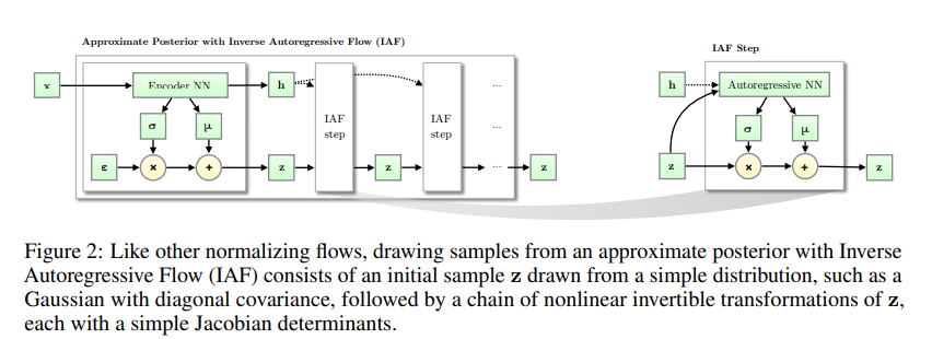
where \( \boldsymbol{\mu_{t}} \) and \( \boldsymbol{\sigma_{t}} \) are outputs of an autoregressive neural network, with inputs \( \mathbf{z_{t-1}} \) and \( \mathbf{h} \). This is shown in the below figure
The autoregressive neural network is structured such that elements of \( \boldsymbol{\mu_{t}} \) and \( \boldsymbol{\sigma_{t}} \) are only dependent on elements of \( \mathbf{z_{t-1}} \) with a lower index than them. This means that the the Jacobians \( \frac{d \boldsymbol{\mu_{t}}}{d \mathbf{z_{t-1}}} \) and \( \frac{d \boldsymbol{\sigma_{t}}}{d \mathbf{z_{t-1}}} \) are triangular with zeros on the diagonal and \( \frac{d \mathbf{z_{t}}}{d \mathbf{z_{t-1}}} \) is triangular with \( \sigma_{t}^{i} \)’s on the diagonal. To see this consider the derivative of a single element of \( \boldsymbol{z_{t}} \) (denoted \( z_{t}^i \) with respect to a single element of \( \mathbf{z_{t-1}} \) (denoted \( z_{t-1}^j \) ).
\begin{equation} \frac{d z_t^i}{d z_{t-1}^j} = \frac{d \mu_t^i}{d z_{t-1}^j} + \frac{d \sigma_t^i}{d z_{t-1}^j} \times z_{t-1}^j + \frac{d z_{t-1}^i}{d z_{t-1}^j} \times \sigma_t^i \end{equation}
now if i < j, all of the above terms are 0. This means that the matrix is triangular, and the jacobian determinant of a triangular matrix is just the diagonal columns. This means we only have to fucus on the derivatives for i = j. For i = j, bothe of the first terms of the above equation become 0 (as \( \sigma_{t}^i \) and \( \mu_{t}^i \) are only functions of \( z_{t-1}^{1:i-1} \). Thus we get
\begin{equation}
\begin{aligned}
\frac{d z_t^i}{d z_{t-1}^i} &= \frac{d \mu_t^i}{d z_{t-1}^i} + \frac{d \sigma_t^i}{d z_{t-1}^i} \times z_{t-1}^i + \frac{d z_{t-1}^i}{d z_{t-1}^i} \times \sigma_t^i
&= 0 + 0 + 1 \times \sigma_t^i
\end{aligned}
\end{equation}
and therefore the determinant is simply given by \( \prod_{i=1}^{D} \sigma_t^i \). Thus the density under the final iterate is,
\begin{equation} \log q\left(\mathbf{z_{T}} \mid \mathbf{x}\right)=-\sum_{i=1}^{D}\left(\frac{1}{2} \epsilon_{i}^{2}+\frac{1}{2} \log (2 \pi)+\sum_{t=0}^{T} \log \sigma_t^i\right) \end{equation}
Why IAF?
IAF scales better to high dimensional datasets than other normalising flows. The autoreggressive NN allows an expressive transformation to be applied during each step, where complex relationships between elements can be introduced. For example, the final element of \( \mathbf{z_t} \), denoted \( z_t^N \), is a function of \( \mathbf{z_{t-1}^{1:N-1}} \), the second last element of \( \mathbf{z_t} \), denoted \( z_t^{N-1} \), is a function of \( \mathbf{z_{t-1}^{1:N-2}} \) - thus the last and second last element may have a complex relationship/dependence, through their shared (but different) dependence on \( \mathbf{z_{t-1}^{1:N-2}} \). The relationship of these elements is rich because the deep neural network mapping inputs to autputs is expressive. Lastly, we note that these complex dependencies are introduced through parellel processes (as NN’s are highly parrellel).
This can be contrasted by the normalising flow transformation proposed in the original normalising flow paper defined as follows:
where \(\mathbf{u}\) and \(\mathbf{w}\) are vectors, \(\mathbf{w}^{T}\) is \(\mathbf{w}\) transposed, \(b\) is a scalar and \(h(.)\) is a nonlinearity. The second term can be seen as a single unit, single layer, multilayer percepton. This function is far less expressive than the autoregressive NN, and requires many sequential steps (not in parellel) to obtain high-dimensional dependensies. Thus we can see that IAF obtains a far richer transformation per step, while maintaining the requirement of having a simple, known Jacobian determinant.
Quick summary of how the autoregressive NN gets its autoregressive-ness
To output i and input j, the autoregressive NN simply blocks connections between nodes that lead from j to i for i < j. To implement this for a deep NN certain nodes are “allocated” to certain outputs (for management of the blocking/ensuring that each input is processes with a sufficient number of nodes), and the blocking is performed using element by element multiplication with a masking matrix (i.e. a matrix with 0’s for connects/weights that should be blocked, and 1’s for connections that are allowed).